If you have read my last article, you know that we have been here before. Although I talked about the process of completing and submitting Project 2, I wanted to write about Project 3 but focus on more of the content I learned from it.
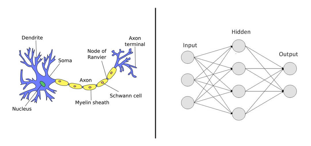
Project 3 was completely different to Project 2- not only in terms of difficulty, but also what it meant it to me. In high school, I remember binging YouTube videos on neural networks for hours upon hours. I thought they were extremely interesting and powerful- but still had no idea how they really worked. Another reason that the algorithm caught my attention firstly was due to the relation the name has to the human brain, which has always fascinated me. Below is a picture that shows the relation between a brain’s neurons and a computer neural network.
Neural networks and their allure were part of the reason that I wanted to study the Intelligence thread as CS major- so this particular project in Machine Learning was going to be important for unveiling the black box of how they work.
What is a Neural Network?
Neural networks seem extremely complicated, and they definitely can be. However, there are simple ways to think about them that makes the understanding much easier. Simply put, a neural network is a set of algorithms working together to show relationships in a dataset and try its best to mimic the behavior of human brains. They represent one of the most popular algorithms and can be programmed to do almost anything.
This particular project was focused on one of the algorithms potential uses- text classification. Text classification is when a computer model is able to categorize words based on a certain trait they possess. For example, for this assignment, we were given the iMDB dataset of movie reviews that the computer model would take in and break down to analyze. The model is also fed training data and testing data- the training data is what the computer uses to learn how things are classified and the testing data is used to test the model’s accuracy. The computer model must be accurate on classifying movie reviews as either positive or negative on both sets of data. The coolest part of implementing a neural network like this is when it can accurately predict whether it is reading a nice review or bad review just like a human.
Neural Bag of Words
For the sake of length, I will only discuss one of the algorithms we implemented for Project 3, Neural Bag of Words. NBOW represents the situation in which a bag contains a bunch of words; think of someone reaching into a bag and fetching a word, but only paying attention to the amount of times a word appears and disregards grammar and word ordering from the word’s original sentence. This means that every single word in the bag is treated the same, it doesn’t matter what the word’s meaning or significance is.
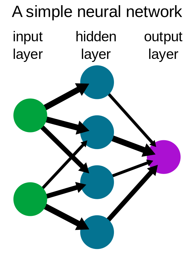
The Neural Bag of Words model works like any other neural network- with an input and output layer, and a hidden layer in between.
This algorithm works its magic by using an embedding layer, which helps convert words to vectors that can be used in the neural network. In our situation the input layer consists of the IMDB review dataset and the output we get is an accuracy of the computer’s prediction on the nature of the reviews.
Conclusion
Although I have only scratched the surface of what a neural network is made up of and does, the message of how strong it can be should be clear. Using neural networks, computer scientists can train any computer to predict anything at all using just an established dataset and training time! The possibilities of functions are endless!
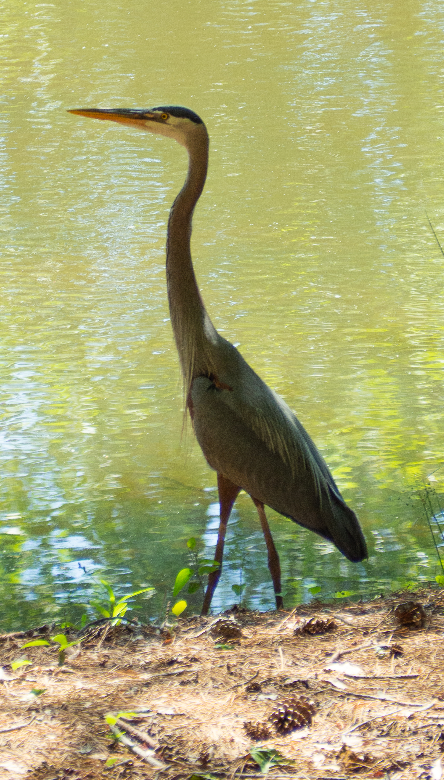
Great blue herons are part of the Ardea genus, which is a genus of birds that includes the herons, egrets, and bitterns. These birds are typically pretty large in size, with lengths usually greater than 80–100 cm. You’re most likely to find members of this genus in wetlands and other partially aquatic habitats.
Feeding Behavior
Great blue herons are carnivores, and they eat a variety of aquatic, semi-aquatic, and terrestrial prey. Their diet consists of predominantly fish, but they will eat pretty much anything that they can catch in their beaks. Fish are supplemented by amphibians, reptiles, small ground mammals, and even other birds. Great blue herons catch smaller prey in the jaws at the back of their beak, although they prefer to stab larger prey with their beaks.
There are 38 total feeding behaviors that have been recorded by members of the Ardea family. Each species in this genus uses multiple feeding methods — they’re creative hunters. Twelve of these strategies have been observed in great blue herons. The most commonly observed feeding behavior for the great blue heron is standing and waiting, where the heron simply stands still and waits for its prey to come to it. Herons also will move slowly, either through the water or through a field, in search of prey. More dramatically, the great blue heron will occasionally plunge-dive, diving down quickly and with force, to catch its prey. A particularly interesting feeding behavior of the great blue heron is to stick its bill in the water, and vibrate it. The underwater vibrations create ripples, attracting fish and other aquatic prey.
Habitat
Great blue herons prefer to live in wetlands, especially when nesting. Rather than nesting alone, great blue herons nest in colonies. Colony nesting is particularly common for birds that live in aquatic environments. Colonies can have over 500 nests (so easily over a thousand birds) all relatively close together. For large scale habitats and especially for colony nesting, great blue herons have preferences for certain types of habitats over others. The lacustrine wetlands is a particular favorite of Illinois great blue herons. Lacustrine wetlands are any wetland or deepwater area that has these three characteristics:
Located in a valley/depression in the ground
Lacking trees, shrubs, and other plant life that covers more than 30% of the area
At least 20 acres in surface area
Biologists believe that herons may prefer this biome for their habitats due to the easy access to their preferred prey of small bodied vertebrates. Additionally, large wetlands tend to be isolated from human activity, which great blue herons tend to avoid if possible.
References
Combs, B. P. (2021). Great Blue Heron Forages for Fish by Bill-Vibrating. Western North American Naturalist, 81(2), 280–284. https://doi.org/10.3398/064.081.0213
Gibbs, J. P., & Kinkel, L. K. (1997). Determinants of the Size and Location of Great Blue Heron Colonies. Colonial Waterbirds, 20(1), 1–7. https://doi.org/10.2307/1521757
Knight, E. C., Vennesland, R. G., & Winchester, N. N. (2016). Importance of Proximity to Foraging Areas for the Pacific Great Blue Heron (Ardea herodias fannini) Nesting in a Developed Landscape. Waterbirds, 39(2), 165–174. https://doi.org/10.1675/063.039.0207
The red-shouldered hawk (Buteo lineatus) is a raptor that is found in forests throughout North America. Year round, the red-shouldered hawk is found throughout much of the Eastern and Midwestern United states. During their breeding season, they can be found in both the northeastern and western United States as well as part of Atlantic Canada. They also have a non-breeding range in Mexico, where they are found for some parts of the year. Red-shouldered hawks can be identified by their medium size and reddish-brown feathers on their chests and shoulders. Hawks from the western part of their range tend to be a deeper red than those found in the eastern part. As for their wings, the feathers are banded black and brown from the underside, with black and red being predominant on the outside. Their tails are also banded, which is another identifying trait of the species.
Sexual Dimorphism in Red-shouldered Hawks
Red-shouldered hawks do show some sexual dimorphism in their appearance. Sexual dimorphism occurs when males and females of the same species show different traits on average, such as average size and weight. Mass is one of the traits that is sexually dimorphic for red-shouldered hawks. Females are larger than males, with the average male being only 85% of the mass of the average female. Researchers recently have tried to establish other ways of determining the sex of red-shouldered hawks morphologically. Determining sex by morphology is used by biologists to guess at the sex of an animal without needing to check for sure with DNA testing. Sex determination based on morphology is more convenient than determining sex based on molecular testing, and can be done by biologists in the field without access to DNA testing equipment. Other features of red-shouldered hawks that are sexually dimorphic are toepad length, length of secondary feathers, bill length, mass, and wing chord length. However, mass remains the most reliable way to morphologically determine the sex of a red-shouldered hawk.
Diet and Habitat of the Red-shouldered Hawk
The diet of the red-shouldered hawk is mostly made up of small mammals, lizards, snakes, and amphibians, and these hawks typically live in riparian forests. Riparian forests are forests that are on or near the bank of a river or stream. There is evidence that the composition of the red-shouldered hawk’s diet varies depending on where in their range they are living. One study split red shouldered-hawks into two groups. The first group was the northern hawks, which live above 38o N latitude. This is the latitude line passing just south of Charlottesville, VA, and through Lexington, KY. Interestingly, northern hawks preferred more mammalian prey and less amphibian prey. The opposite was true for southern hawks. Researchers noticed that diets were more mammalian in drier conditions, whereas hawks that lived in wetter conditions relied more on invertebrate and amphibian prey. It’s possible that hawks that live in drier areas will be less affected by wetland degradation than hawks in wetter areas.
Nesting Preferences of the Red-shouldered Hawk
Where red-shouldered hawks choose to nest is another area of interest for researchers. Typically, red-shouldered hawks prefer to nest in large tracts of mature forest, although they can also be found in more fragmented forested areas, such as those found in suburban areas. One study found that nests were more likely to be located near a lake or treeless wetland than not. Nests were also more likely to be near a trail or stream than not for both cases. Researchers believe that open trails might make good hunting grounds for the hawks, without trees and underbrush to hide prey. We can guess similarly about hawks’ proximity to lakes and treeless wetlands. The lack of trees gives hawks easier access to their prey, which they detect primarily via eyesight. Red-shouldered hawks’ positive association with wet areas is a well known feature – amphibians make an important component of the diet of the red-shouldered hawk, especially while nesting.
References
Cheryl R. Dykstra, Herman L. Mays Jr, Jeffrey L. Hays, Melinda M. Simon, & Ann R. Wegman. (2012). Sexing Adult and Nestling Red-Shouldered Hawks Using Morphometrics and Molecular Techniques1. Journal of Raptor Research, 46(4), 357–364. https://doi.org/10.3356/JRR-11-84.1
Brad N. Strobel, & Clint W. Boal. (2010). Regional Variation in Diets of Breeding Red-Shouldered Hawks. The Wilson Journal of Ornithology, 122(1), 68–74. https://doi.org/10.1676/09-071.1
Landenberger, James F, Roosa, Dean M, Stravers, Jon W, Ehresman, Bruce, & Patterson, Rich. (2013). The Raptors of Iowa. University of Iowa Press.
James E. Woodford, Carol A. Eloranta, & Anthony Rinaldi. (2008). Nest Density, Productivity, and Habitat Selection of Red-Shouldered Hawks in a Contiguous Forest. Journal of Raptor Research, 42(2), 79–86. https://doi.org/10.3356/JRR-07-44.1
Red-shouldered Hawk Overview, All About Birds, Cornell Lab of Ornithology. (2019). allaboutbirds.org. https://www.allaboutbirds.org/guide/Red-shouldered_Hawk/
The Yellow-Bellied Sapsucker: A Well Traveled Woodpecker
A yellow-bellied sapsucker.
The yellow-bellied sapsucker (Sphyrapicus varius) is a woodpecker that has a wide range across North America. In summer, the sapsucker can be found as far north as Alaska, Minnesota, and Nova Scotia and in winter, the birds can be found as far south as much of Central America and the Caribbean. The yellow-bellied sapsucker is migratory — the birds spend the winters in the south, and their summers in the north. This is unusual for woodpeckers. Out of the twenty two woodpecker species found north of Mexico, fifteen of them don’t migrate at all, with many of these species only flying for short distances during their regular activities. This leaves us with seven woodpecker species that do migrate — and of those, the yellow-bellied sapsucker takes the crown for the largest migration range. Interestingly, the sapsuckers do their migratory flying at night.
Yellow-Bellied Sapsucker Habitat and Diet
The yellow-bellied sapsucker is found in forests. Maple forests, aspen forests, and mixed forests are all popular habitats for sapsuckers. Research has shown that maple forests have better outcomes overall for breeding sapsuckers than aspen forests. However, both maple and aspen forests allow sapsuckers to sustain their populations over time. Both of these forests have trees that are good for sap drilling — the yellow-birch in maple forests, and the paper birch in aspen forests. Sap is one of the primary food sources of the yellow-bellied sapsucker (which, given the name, isn’t very surprising). Sapsuckers have a variety of preferences for trees to tap for sap depending on their range. In urban areas of Southern Florida, for example, black olive and tropical almond trees are a preferred source of sap. Yellow-bellied sapsuckers also feed on arthropods (think of spiders, centipedes, insects, and the like), especially while nesting.
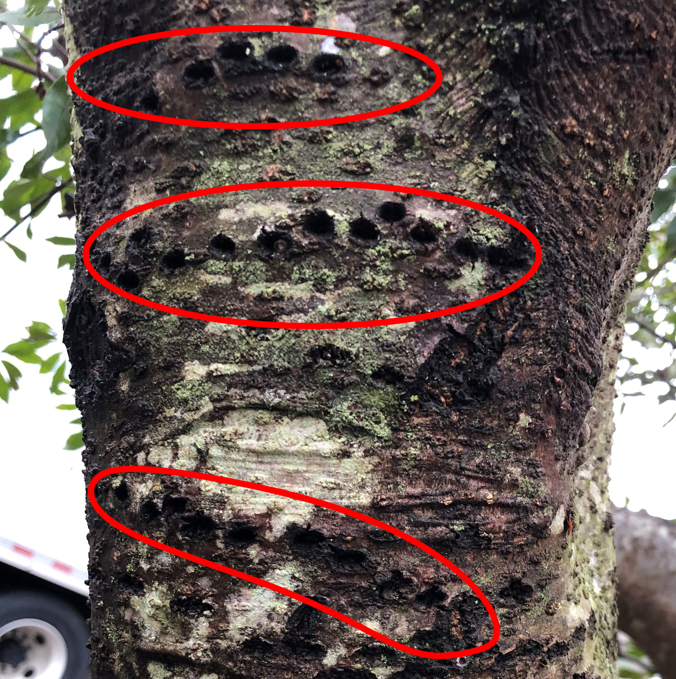
Pictured: Sapsucker holes in a tree. Drilling holes in straight lines is typical for them.
Why are woodpeckers so concussion proof?
One of the most interesting behaviors woodpeckers exhibit as a group is the tree drilling that they’re named for. A very common question related to this drilling is how do woodpeckers avoid rampant brain injuries due to ramming their heads against trees repeatedly, at high speeds, for ages. Woodpeckers routinely bash their heads into trees at far more than double the acceleration that would concuss humans. While humans are concussed at 300 g of acceleration, woodpeckers have been known to regularly drill into trees at accelerations on the order of 600–1500 g.
A variety of mechanisms have been proposed to explain the woodpeckers’ resilience to brain injury. There are three primary reasons woodpeckers aren’t all concussed all of the time. The first being their small size. The acorn woodpecker’s brain, for example, has a mass of 2.5 grams. A human brain has a mass of 1400 grams. The woodpecker brain is so much smaller than a human brain that they generate much less force when they smack into the skull. The second limiting factor that protects woodpeckers is the short duration of impact. One of the documented factors that increases the likelihood someone will be concussed is how long their brain is exposed to high acceleration. A woodpecker only drills against a tree for a millisecond or less each time, so their time of impact is very short.
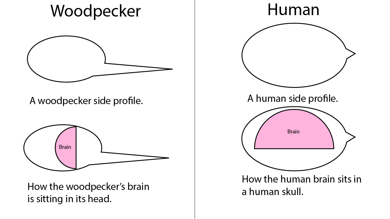
The last quirk of woodpecker anatomy guarding them from brain injury is how their brain sits in their skull. Both human brains and woodpecker brains are hemispherical (if you cut a globe in half, you will have two hemispheres). If you cut the globe in half at the equator, your top hemisphere is oriented like a human brain is. If it were to go flying forward, only the small portion at the front will hit the skull. This concentrates the impact right around the forehead area. On the other hand, a woodpecker brain is much more like if you had cut your globe from the Arctic to Antarctica, and chose to look at the left section. The large flat side of a woodpecker’s brain rests against the front of their skull. When their brain goes smacking against their skull while they drill, the force is distributed among the largest possible region of their brain. This lessens the impact overall.
Notice the difference in alignment when comparing a human brain to a woodpecker brain.Look at how much more relative space the force has to distribute itself on the woodpecker’s brain versus the human brain.
Ecological Status of the Yellow-Bellied Sapsucker
Ecologically speaking, the yellow-bellied sapsucker is in a good place to stick around. The International Union for Conservation of Nature (IUCN) has marked the yellow-bellied sapsucker as a species in the “least concern” of going extinct. Despite this, there are still some concerns for the sapsucker, especially as they’re being seen more and more often in urban and suburban areas. Being in areas with humans presents several new challenges for sapsuckers. Flying into windows is one of these concerns. Some research has been done into this phenomenon, known as “window strikes”. One study suggests that migrating birds are at a higher risk of striking windows than year-round resident birds, which poses a threat for migratory birds like the yellow-bellied sapsucker. Another threat to sapsuckers in areas with high human density are pets, domestic cats in particular. Outdoor cats have long been a threat to bird populations, and sapsuckers living in areas with them are no exception. Like many other species, the yellow-bellied sapsucker’s future will be strongly impacted by human activity.
References
Diamond, Joshua M, & Ross, Michael S. (2018). Tree selection and foraging height of wintering Yellow-bellied Sapsuckers (Sphyrapicus varius) in an urban environment. The Wilson Journal of Ornithology, 130(4), 932-939.
Gibson, L. J. (2006). Woodpecker pecking: How woodpeckers avoid brain injury. Journal of Zoology (1987), 270(3), 462-465.
Natola, Libby, & Burg, Theresa M. (2018). Population Genetics and Speciation of Yellow-Bellied, Red-Naped, and Red-Breasted Sapsuckers (Sphyrapicus varius, S. nuchalis, and S. ruber). The Journal of Heredity, 109(6), 663-674.
Sabo, Ann M, Hagemeyer, Natasha D G, Lahey, Ally S, & Walters, Eric L. (2016). Local avian density influences risk of mortality from window strikes. PeerJ (San Francisco, CA), 4, E2170.
Tozer, Douglas C, Nol, Erica, & Burke, Dawn M. (2011). Quality of mature aspen and maple forests for breeding Yellow-bellied Sapsuckers (Sphyrapicus varius). Canadian Journal of Zoology, 89(2), 148-160.
I am just old enough to remember a time when most textbooks only spoke of exoplanets (i.e. those outside our solar system) in the hypothetical sense, their existence taken as an assumption rather than demonstrable fact, while the question of whether our 8-planet solar system was typical or an anomaly remained a hotly-debated topic. Despite over a century of attempts and subsequent erroneous claims, it wasn’t until 1992 that the first confirmed exoplanet was discovered, two of them as a matter of fact, orbiting the pulsar PSR B1257+12. As surprising as this was to the scientific community, the high likelihood that the planetary pair had formed as the result of a merger between two white dwarfs rather than a collapsing gas cloud meant the world would have to wait another 3 years for the confirmation of a “true” planet orbiting a main-sequence star like the Sun. The discovery ushered in a new era for astronomy and as of November 1st, 2020 there have been a whopping 4,370 exoplanets confirmed in 3,230 star systems. This menagerie of other worlds, ranging from “hot Jupiters” and lava worlds to gas and ice giants and seemingly everything in between stands in stark contrast to the apparently silent heavens, leaving a profound question unanswered:
“Where is everybody?”
Despite what many a crackpot relative or internet crank will tell you, humanity is, to the best of our knowledge, completely and utterly alone in a universe so vast it defies comprehension, a contradiction commonly referred to today as The Fermi Paradox. The concept of aliens and the foundations of the Fermi Paradox have been around for a surprisingly long time, entering the Western conscience with the speculation of Epicurean philosophers like Democritus of ancient Greece, who today is famous for the first conception of atoms. From the viewpoint that the world was merely a chance jostling of these atoms, they argued it was not only reasonable, but exceedingly likely that there exist other inhabited worlds similar to our own. To paraphrase the argument: “who ever heard of a single ear of wheat growing alone in a vast, fertile field?”
Should you happen to see this mentioned on the next episode of Ancient Aliens, it’s worth noting that Democritus’s ideas about “aliens” (and atoms) are not quite as modern as they sound, instead more akin to our modern idea of beings from “parallel universes”, not habitable planets orbiting other stars since the ancient Greeks had no idea what stars and planets actually are, much less orbits. To them, these other worlds existed but were forever inaccessible to us. What’s important is that the core idea, that it’s improbable that life should arise on Earth and only on Earth begins here. Its dismissal by the Aristotelians, who preferred what can be known to what might be and whose influence on Western culture remains to this day, caused such discussion to take a back seat during the early Middle Ages, but the idea remained nonetheless, never being fully dismissed as “impossible” by theologians who were wary of placing what they saw as limits on the omnipotence of the Christian God. Contrary to the popular misconception that discussion of such matters would get one labeled a heretic and burned at the stake, the idea of aliens inhabiting other worlds within our universe that were, at least in theory, accessible to us in some way first arose in the Western world during the late Middle Ages. In his influential work De Docta Ignorantia (1440), Nicholas of Cusa argues that:
Life, as it exists on Earth in the form of men, animals and plants, is to be found, let us suppose in a high form in the solar and stellar regions. Rather than think that so many stars and parts of the heavens are uninhabited and that this earth of ours alone is peopled – and that with beings perhaps of an inferior type – we will suppose that in every region there are inhabitants, differing in nature by rank and all owing their origin to God, who is the center and circumference of all stellar regions (II, p. 12).
His work sparked intense discussion among Christian theologians over whether or not such aliens had been “redeemed” and even whether “original sin” would apply to them. After all it was probably a safe assumption that they were not descended from the mythical Adam and Eve.
The idea stuck around and was eventually taken up by the scientists of the modern era, including the likes of none other than Harlow Shapley who stated in an interview for The Sydney Morning Herald (1959) that:
The universe has 10 million, million, million suns similar to our own. One in a million has planets around it. Only one in a million million has the right combination of chemicals, temperature, water, days and nights to support planetary life as we know it. This calculation arrives at the estimated figure of 100 million worlds where life has been forged by evolution (p. 5)
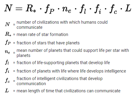
Five months later, Frank Drake performed the first systematic search for extraterrestrial intelligence by monitoring two nearby sun-like stars, 6 hours per day for four months, searching for radio signals around the emission frequency of neutral hydrogen, the most common element in the universe. The reason for this frequency choice is simple: if somebody out there wants their message to be heard, they’ll put it where everyone is already looking. A year later, while preparing to host a meeting for SETI to discuss the future potential of such search efforts, he penned the equation which would bear his name.
Though initially conceived as little more than a mathematical conversation piece, The Drake Equation (as it came to be known) at last allowed astronomers to estimate the number of intelligent civilizations within our galaxy, for the first time couching the discussion in numbers rather than idle speculation. The only problem? Nobody had any real idea what any of these numbers actually were.The various numbers proposed at the meeting by Drake and his colleagues as an “educated guess” give a final value somewhere between a minimum of 20 and a maximum of 50,000,000. Such an enormous range perfectly illustrates their aforementioned uncertainty. In the six decades since, the data from countless observations, surveys, and space missions from NASA, ESA, and observatories around the world have finally shed some light on a few of these parameters which, in theory, allow us to narrow down the estimates a bit.
Mean Rate of Star Formation, R*
Our first parameter in the Drake Equation is R*, the average rate of star formation. For our purposes here, we are only looking for life within our own galaxy so we will use the rate of star formation in the Milky Way. Calculations from the available data suggest that somewhere between 0.68 and 1.45 solar masses of galactic material goes into making new stars every year. To find the star formation rate, we need to also account for the average mass of new stars using the available empirical data which indicates a value of around two stars per solar mass worth of material. Multiplying these two numbers together gives us a value between 1.5 and 3 new stars per year formed in our galaxy, a value slightly higher than the original 1961 estimate of 1 per year.
R* = 1.5 – 3
The Fraction of Stars that have Planets, fp
As mentioned previously, the exoplanet surveys thus far found 3,230 star systems that contain planets. However this figure only tells us the number of stars that have been found to possess planets, not the fraction of them that do. The total number of stars surveyed is much larger at over half a million. Dividing the two numbers gives a value for fp of less than 1%.At first glance, this looks pretty dismal, but there are some important caveats that we need to account for. The majority of exoplanet discoveries were made using the transit method, which makes continuous observations of a star’s light to look for periodic dimming caused by a planet passing in front of it directly along our line of sight. Our chances of observing such dimming is directly related to the star’s radius (bigger is better) and inversely related to the planet’s orbital distance from its host star (closer is better). Should our line of sight to a given system happen to be anything other than virtually edge-on, the transit method will not detect any planets there, even if there actually are. For those that we are fortunate enough to be observing nearly edge-on, if a planet’s orbit is too wide then it will not pass in front of the star from our perspective, thus there will be no dimming and the planet will go undetected. Finally, if a planet is too small, then the star’s dimming could be too small for our instruments to detect and the planet will go undetected.
It perhaps seems that we’re out of luck on getting any reasonable estimates, but statistical analysis of the transit data combined with that of surveys using other methods of planet detection such as doppler spectroscopy and gravitational microlensing point towards a conclusion that even the optimists of the 1960’s would consider absolutely astonishing; fp may very well approach 1, far larger than the maximum estimated value of 0.5 made 60 years ago! In other words, it’s possible that nearly every single star in our galaxy has one or more planets!
fp ≈ 1
Thus far things are looking better than ever for the potential development of intelligent, detectable civilizations (IDCs) in our galaxy, only deepening the paradox. However from here on our estimates for successive factors in the Drake Equation become increasingly speculative.
The Fraction of Potential Life-Supporting Planets that Develop Life, fl
This number is even more difficult to estimate than the previous factor. Our current sample size for life-supporting planets that go on to develop life is 1, with a possibility of 5 more if Mars, Venus, Titan, Europa, and/or Enceladus are eventually found to have or have had life. Some scientists argue that life arises as a rule virtually as soon as conditions are right, so this value should be ‘one’. Others argue it may actually be a freak occurrence even in all the right conditions, so this number should be tiny. In the case of our planet, life appears to have developed as soon as the conditions were right, but any attempt to extrapolate this to other planets contains heavy anthropic bias as our model planet (Earth) was not chosen randomly but rather by the organisms already inhabiting it. There currently is no evidence that abiogenesis occurred more than once on Earth, yet if it were a common phenomenon we might reasonably expect it to have occurred several times. It certainly could have, but all known terrestrial life shares a common origin, meaning if it ever did then those lineages are most likely long gone. If abiogenesis does indeed turn out to be an incredibly rare event, there is still a potential loophole. Remember, we only care about the number of habitable planets that go on to actually develop life, not how that life got there in the first place. It is entirely conceivable that planets, including our own, could have been seeded with microbial life that hitched a ride on a rogue piece of post-collision debris ejected from another already inhabited planet, a hypothesis known as panspermia. A technologically advanced civilization could also choose to do this intentionally in order to spread its genetic family throughout the galaxy. It may sound far-fetched, but humanity already has the capability to do this. Scientists and engineers go to painstaking lengths to sterilize spacecraft in order to avoid unintentionally ‘infecting’ other planets or moons with potentially invasive extremophile Earthlings. The various proposed panspermia hypotheses are a topic that honestly deserve an article all their own, so for now we will wrap things up optimistically and use the original estimate made by Drake and his colleagues back in 1961.
fl ≈ 1
You may have noticed we skipped over a factor, the average number of habitable planets per star with planets. Like panspermia, this factor warrants its own discussion and is the subject of part two in this series. Stay tuned!
Osedax, from the Latin os, oris (bone) and edāx, edācis (devourer), is a genus of undersea worms that consumes bone. A genus (which is more Latin, this time for a family group) is a group of species that are similar. More distantly, the genus Osedax belongs to the family Siboglinidae. Siboglinidae is a family (a level above in the biological categorization hierarchy from genus) composed of segmented worms, all of which have chitin bristles. Chitin is a natural substance that is found in all sorts of bugs, and it’s similar to the material that makes up your fingernails. Another prominent species in this family are the undersea tubal worms that live at the hydrothermal vents at the bottom of the ocean. It turns out there is a surprising amount of diversity of species of undersea bone eating worms. The worms range in size and in behavior. You can find members of the Osedax genus in all seven oceans, and in all sorts of depths (21 – 4000 m). Some of them are generalists, whereas others specialize in large bone deposits often found on the ocean floor. Whalefalls (you can read more about them here: http://chargedmagazine.org/2012/06/whale-fall-2/) are one such source of large bone deposits on the ocean floor.
Osedax worms were first discovered in 1994. Biologists were initially baffled at what exactly they were. The worms evaded classification until molecular DNA analysis showed that they were related to the tube worms that live in hydrothermal vents on the ocean floor. This breakthrough allowed biologists to finally place the Osedax genus into the Siboglinidae family. Later, fossils were discovered of Osedax worms inhabiting a large, dead reptile, dated to the early-Late Cretaceous period, about 100 million years ago. This led to several revelations about the history of Osedax worms. Firstly, there was now a historical precedent for being generalists, rather than whale specialists. Osedax worms were initially discovered and identified on whale falls, and there was some debate in the scientific community about whether or not they occupied other niches. Well, giant dead reptiles certainly weren’t whales, so this find cleared that up nicely. The fossil finding also illustrates something about the history of Osedax worms and the Siboglinidae family. This finding confirmed an earlier theory that the Siboglinidae family originated somewhere in the mid-Cretaceous period. It also means that the weird bone eating worms under the sea outlasted the dinosaurs, which is neat.
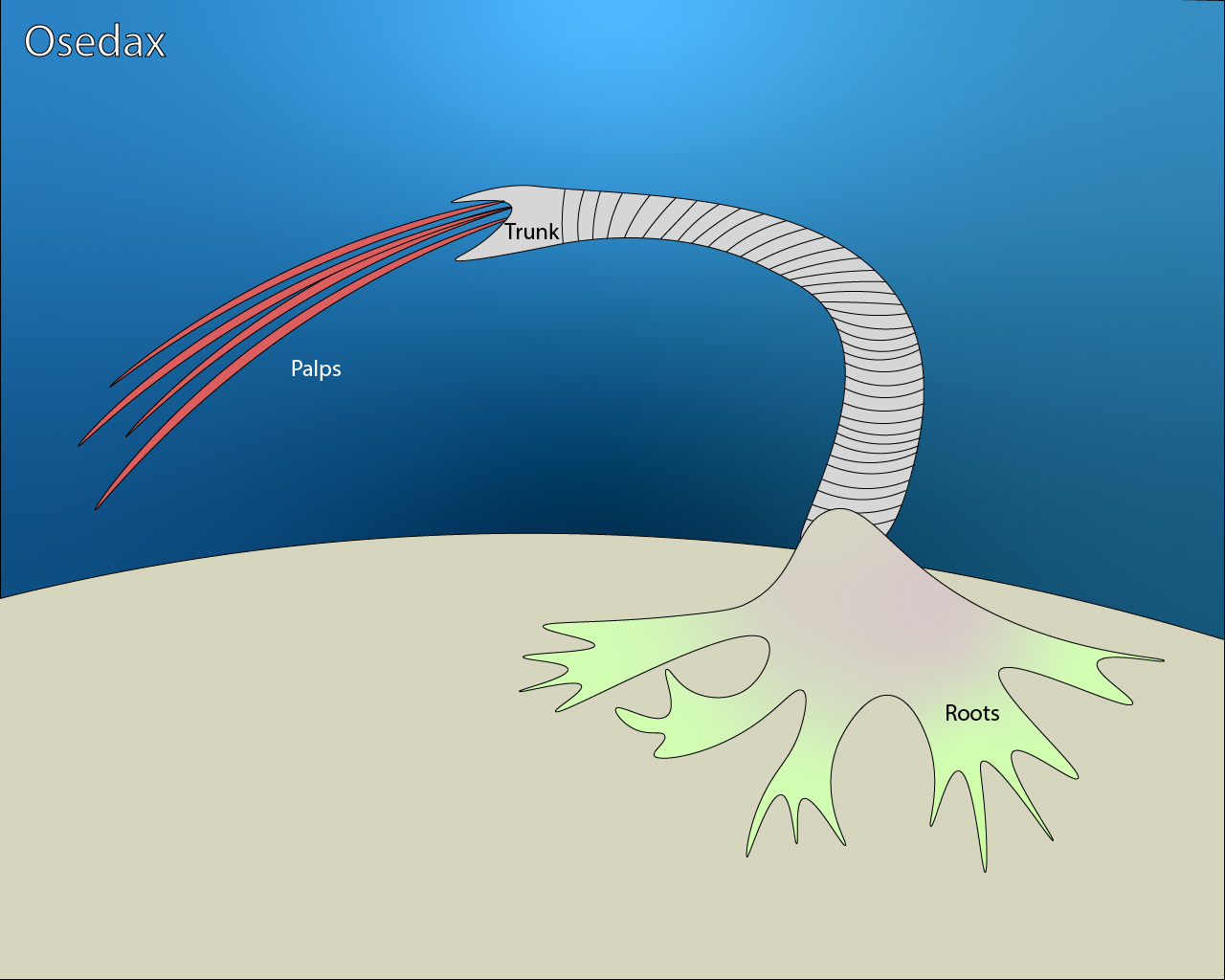
A labeled illustration of an Osedax worm.
Physically, Osedax worms are strange looking creatures. Red, string-looking bits float out from one side of the main worm body. On the other side, there are green, root-like structures sticking out back. These roots secrete acids to dissolve the bones where they lodge. Their middle is a white, segmented tube. It doesn’t get any more regular on the inside, either. Osedax worms don’t have a digestive system – they just host a wealth of bacteria inside of them to digest the bones they consume. Another strange thing about the inside of an Osedax worm is that the male worms live inside the females. As in, every picture of an Osedax worm you see will be of a female, as the males are teeny tiny and live inside of the females. Dwarf males, as this phenomenon is called, occurs when the males of a species are much smaller (and usually simpler anatomically) than the females. In species where dwarf males exist, the males typically reside somewhere inside or attached to the female members of the species. Osedax worms are at least as odd as you were expecting worms that ate bones to be, at very least.
References
Smith, Craig R, Glover, Adrian G, Treude, Tina, Higgs, Nicholas D, & Amon, Diva J. (2015). Whale-Fall Ecosystems: Recent Insights into Ecology, Paleoecology, and Evolution. Annual Review of Marine Science,7(1), 571-596.
Rouse, G. W. (2004). Osedax: Bone-Eating Marine Worms with Dwarf Males. Science (American Association for the Advancement of Science),305(5684), 668-671.
Danise, S, & Higgs, N. D. (2015). Bone-eating Osedax worms lived on Mesozoic marine reptile deadfalls. Biology Letters (2005),11(4), 20150072.
In the fitness community, novice and expert athletes alike, are continually searching for supplements that will give an athletic edge in their workouts. There are many athletes, especially newer and younger ones, that are ingesting supplements without actually understanding what the supplements are doing to their bodies. Since workout supplements are not regulated by the US FDA, manufacturers are able to put whatever they want into their supplements – even ingredients that toe the line between legal and illegal, including some ingredients that are amphetamine derivatives. These manufacturers hide these ingredients in what they call “proprietary blends”. So that you can be informed, here are the three most common and generally accepted to be safe workout supplements:
1) Creatine
2) Caffeine
3) Beta-Alanine
Additionally, these are two ingredients in popular supplements today that you should NOT be taking:
1) DMAA
2) DMHA
This is an example of a nutrition label of a pre-workout supplement. Always look at the supplement facts to see what ingredients your supplement contains!
Supplements Generally Accepted to be Safe
Creatine
Creatine is one of the most popular supplements used by athletes looking to build lean muscle mass, maximize athletic performance, and increase strength. Typically, creatine is in the form of creatine monohydrate, a nitrogen-containing compound that can be obtained in the food we eat – from sources like meat and fish – or formed endogenously (or inside the body), from three specific amino acids: glycine, arginine, and methionine.
Creatine helps in the production and recycling of ATP. Adenosine Triphosphate, or ATP, is an organic compound responsible for being the main source of energy for essentially all bodily processes. Whether you’re running, lifting weights, or even carrying groceries inside, your body is consistently using ATP to produce energy. After your body uses ATP for energy, the chemical bi-product produced is adenosine diphosphate, or ADP. Your body then begins the process of recycling ADP back into ATP.
With the help of creatine, ADP recycling is exponentially increased, improving muscular endurance and power. There have been over 300 scientific studies highlighting the effectiveness of creatine. In fact, over 70% of these studies show statistically significant results in muscle growth and performance while taking creatine over an 8-week period of time. In the fitness world, fitness experts advise taking 20mg of creatine monohydrate for about 1 week to saturate your cells with creatine. From there, you can reduce your intake to 5mg per day. Although supplementing with creatine doesn’t guarantee muscle growth and athletic improvement, it can certainly help with overall energy production in the body, if you supplement correctly. A potential drawback to creatine is that it has been shown to be hard on kidneys, especially in people with pre-existing conditions. However, as always, you should consult your physician before starting new supplements. If you consult with your physician and supplement correctly, you can gain the benefits of using creatine in your workouts!
Caffeine
Ahh, caffeine – a familiar word to pretty much every student on a college campus (and probably to high school students). Caffeine takes many forms, whether you imbibe yours with coffee or espressos, or you take yours in a pill form. Caffeine is the world’s most popular central nervous system stimulant and performance-enhancing supplements. It has become such a prolific supplement that it seems the world runs on caffeine.
In fact, supplementing with caffeine has been scientifically proven to have significant ergogenic effects on aerobic and anaerobic activities (think endurance and sprinting, respectively).
Caffeine is able to give you that desired jolt of energy by activating adenosine receptors in your brain. Consequently, dopamine floods your brain and causes increased neuron firing. The pituitary gland senses this activity and stimulates your flight-or-fight response, causing your body to release adrenaline. This chemical cascade is why caffeine makes you feel awake and energized. Caffeine acts as a muscle and chemical stimulant as well as a brain stimulant.
While working out, caffeine can empower your body to push through even the hardest workouts, while keeping you focused on getting your next weightlifting or running personal record. Most workout supplements will have 120 – 180mg of caffeine per serving. Taking caffeine in the appropriate amounts can push you through your workout. However, since workout supplements are not FDA regulated, some supplements will include over 500mg of caffeine, claiming to give you the best workout of your life. However, healthy adults should not consume more than 400mg of caffeine per day – actually, it’s quite unsafe and unhealthy to consume more. So, when you go to take your next workout supplement, make sure to check the nutrition label for how much caffeine it includes and be sure that taking it doesn’t interfere with your morning cup of coffee or tea!
Beta-Alanine
If you use workout supplements, especially pre-workout supplements, you’ve most likely heard of Beta-Alanine. Beta-Alanine is a non-essential amino acid that is produced naturally in the body. In the body, Beta-Alanine aids in the production of carnosine. Carnosine is important for many normal body functions including the proper function and development of your muscles, heart, liver, kidneys, brain, and other organs. The exercise world focuses on carnosine’s role in muscle endurance in high-intensity exercises, such as weightlifting.
Since Beta-Alanine helps in the production of carnosine, supplements typically include Beta-Alanine in pre-workouts geared for weightlifting or other high impact exercise activities. Because carnosine is specifically linked to muscle endurance, it is thought to help create longer weightlifting workouts, in turn leading athletes to true muscle exhaustion, consequently leading to muscle growth.
Although science generally supports Beta-Alanine’s support in the creation of carnosine, there is still quite a bit of research that needs to be undertaken to verify the efficacy of the supplement. In general, the recommended effective and safe dose for Beta-Alanine is around 3-6 grams. Taking more is not advised as the safety effects of taking more have not been proved to be more effective nor safe. Interested readers should be cautious, however, when taking this supplement. Beta-Alanine can cause a tingling sensation in their body, called paresthesia. This tingling sensation stems from central nervous system stimulation and muscle stimulation. Though completely harmless, people that are sensitive to these kinds of body effects should either reconsider taking Beta-Alanine or take it in lower doses to assess tolerance.
In general, Beta-Alanine is a great, generally safe supplement to use in sports and weightlifting. As always, consulting your physician is always smart before starting any new supplement. However, users in good health are generally safe and benefit from taking Beta-Alanine in supplementing for their workouts.
Supplements you should not be taking:
DMAA
1,3 Dimethylamylamine (a.k.a. 1,3-DMAA or DMAA) is a substance made synthetically in laboratories. Surprising, it was originally used as a nasal decongestant in medicines from around the 1960s. Today, 1,3-DMAA is sold as a dietary supplement for a myriad of reasons including ADHD, weight loss, and improving athletic performance, as DMAA is classified as a stimulant. Many athletes take 1,3-DMAA to improve performance, without understanding the effects on the body.
However, it was determined that DMAA is chemically too close to drugs and controlled substances like certain amphetamines – it even causes failures on drug tests for drug-tested athletes. Consequently, DMAA was added to the World Anti-Doping Agency’s prohibited substances list in 2010. Its use has been linked to several reports of serious, life-threatening side effects. You definitely should stay away from any workout supplement that includes this in their proprietary blend or ingredient list!
DMHA
Like DMAA, 1,5-Dimethylhexylamine (DMHA) was originally used as a drug for nasal congestion, similar to drugs such as pseudoephedrine, etc. Today, DMHA is included as an ingredient in dietary supplement products to supposedly boost workout performance or for weight loss. DMHA is very close to DMAA, but unlike DMAA, DMHA is currently not illegal. However, because of its close relation with DMAA and other amphetamines and controlled substances, many professional athletic communities actively advise against using any supplement with DMHA (i.e. NCAA for US college sports). While DMAA is a very potent stimulant that will definitely make even the hardest workouts feel ‘easy’, there are no studies to show the safety of DMAA, and there have even been reports of severe side effects from ingesting DMAA. If you see a workout supplement that includes DMAA, you should definitely not take it!
NSF label
When in doubt, check for the NSF label!
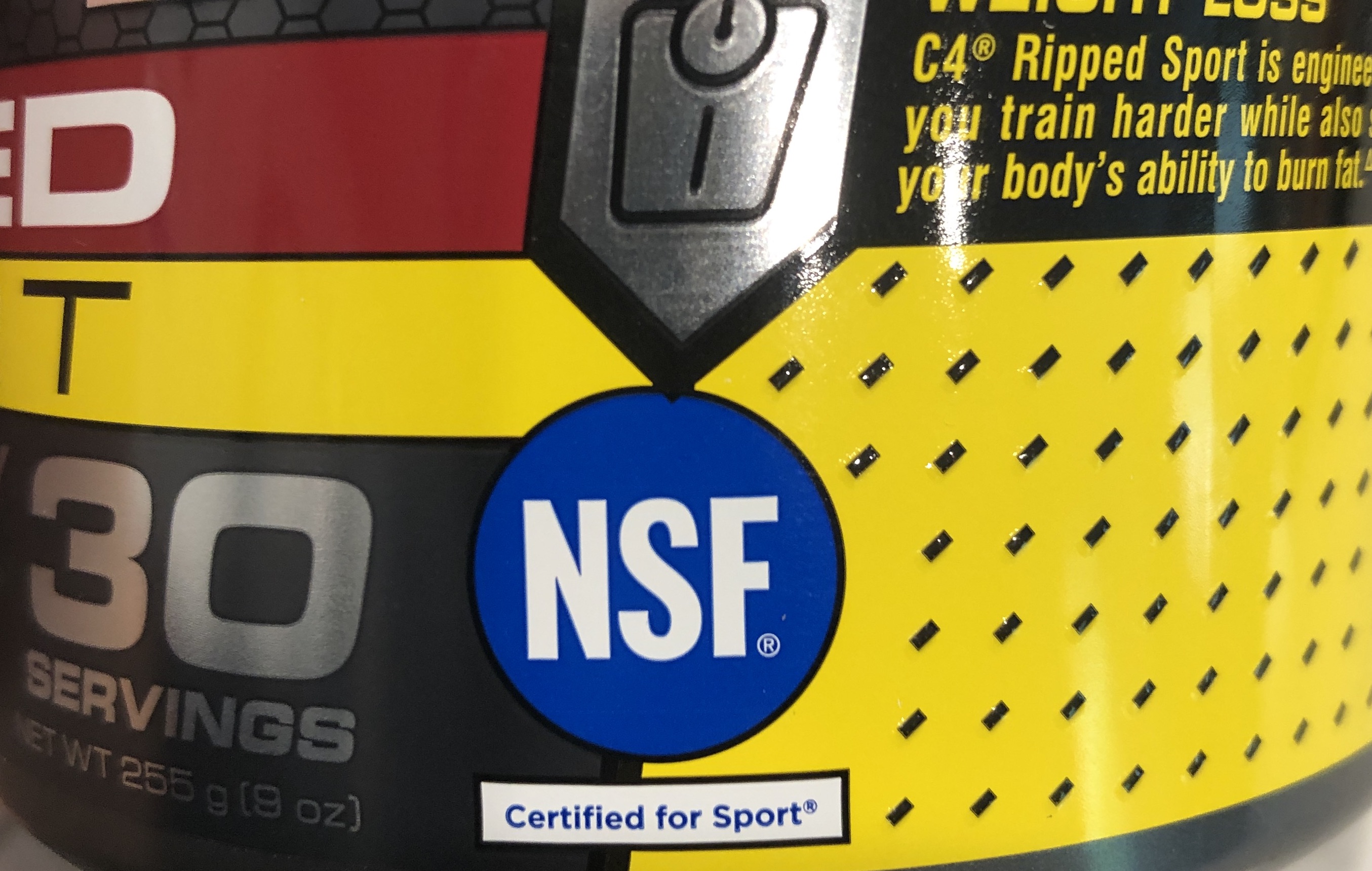
If you doubt your ability to check a supplement’s ingredient list, it’s always a good idea to check if the product has an NSF label. NSF is the National Sanitation Foundation which was established to standardize food safety requirements. This organization is composed of chemists, biologists, nutrition experts, doctors, and more, who test and validate sports supplements (among other products) for their safety and efficacy. In fact, the U.S. NCAA mandates that athletes only take workout supplements with the NSF label, as this ensures the product does not contain any banned or harmful substances. If you choose a product that has the NSF label, you can be sure that the supplement is scientifically proven to be effective, generally accepted to be safe to use, and will not have any banned substances of any kind.
Ask your physician and go crush your workout
Now that you are aware of the more popular “generally accepted to be safe” supplements, as well as the supplements that you shouldn’t take, I hope that you are more informed when it comes to decisions about the supplements you take. In general, you should not begin taking new supplements until you have consulted with your physician. This article is by no means seeking to give advice; this article only seeks to bring awareness. Now get out there, be safe with your supplements, and crush your next workout!
Notice: Pictures featured in this article are not to be considered an endorsement of that specific product.
Sources:
Kreider, R. (2003, February). Effects of creatine supplementation on performance and training adaptations. Retrieved November 01, 2020, from https://pubmed.ncbi.nlm.nih.gov/12701815/
Grgic, J., Trexler, E., Lazinica, B., & Pedisic, Z. (2018, March 5). Effects of caffeine intake on muscle strength and power: A systematic review and meta-analysis. Retrieved November 01, 2020, from https://www.ncbi.nlm.nih.gov/pmc/articles/PMC5839013/
Ratini, M. (2019, January 30). Beta-Alanine: Uses and Risks. Retrieved November 01, 2020, from https://www.webmd.com/vitamins-and-supplements/beta-alanine-uses-and-risks
NIH. (2019). Paresthesia Information Page. Retrieved November 01, 2020, from https://www.ninds.nih.gov/Disorders/All-Disorders/Paresthesia-Information-Page
WebMD. (2018). 1,3-Dmaa: Uses, Side Effects, Interactions, Dosage, and Warning. Retrieved November 01, 2020, from https://www.webmd.com/vitamins/ai/ingredientmono-1258/1-3-dmaa
WebMD. (2018). Dimethylhexylamine (Dmha): Uses, Side Effects, Interactions, Dosage, and Warning. Retrieved November 01, 2020, from https://www.webmd.com/vitamins/ai/ingredientmono-1538/dimethylhexylamine-dmha
Electric vehicles have gained momentum in the recent years due to a considerable percentage of personal vehicle users as well as freight companies that converted from using internal combustion engine vehicles to some type of electric vehicles. Electric vehicles by definition, have at least some electric powerplant that powers the engine particularly or completely by one or more electric motors. This article forces on the environmental impacts of electric vehicles that entirely depend on batteries for storage and delivering electric power for the motors.
Plug-in hybrid electric vehicles (PHEVs) are being developed for a decade or so for mass production by the automotive industry by some major automakers. However, the rise of Tesla, the most valued automaker at the moment during the time of writing this article, have pushed the limit of how an average car user can adopt completely to an all electric car and thereby save the environment from massive carbon footprint resulting from fossil fuels. PHEVs do not use any type of fuel other than battery packs that store and deliver energy. PHEVs have been touted for their potential to reduce the transportation system’s petroleum dependence and greenhouse gas emissions by using off-peak excess electric generation capacity and increasing the vehicle’s energy efficiency. As such, PHEVs are in a massive boom as several other companies have emerged with large financial backings that have pledged to produce EVs to save the environment and to ensure a zero emission transportation system in the future. The burning question is of course: do EVs actually have a significant impact in the improvement of environment?
The U.S. Department of Energy’s has a Vehicle Technology Program that examines the precompetitive, high-risk research needed to develop the component and infrastructure technologies necessary to enable a full range of affordable cars and light trucks that are expected to reduce the U.S. dependence on imported oil and minimize harmful vehicle emissions, without sacrificing freedom of mobility and freedom of vehicle choice [1]. Although PHEVs are similar to the regular hybrid electric vehicles (HEVs), the battery can be charged using electricity from the grid by being recharged through a wall outlet. In terms of the overall environmental impact, PHEVs not only have direct impact as a result of not burning traditional fuels, but also the battery chemistry, the amount of grid electricity that can be stored in the battery, recycling ability of the raw materials, and the ability to give unused “power back to the grid” could significantly impact the environment.
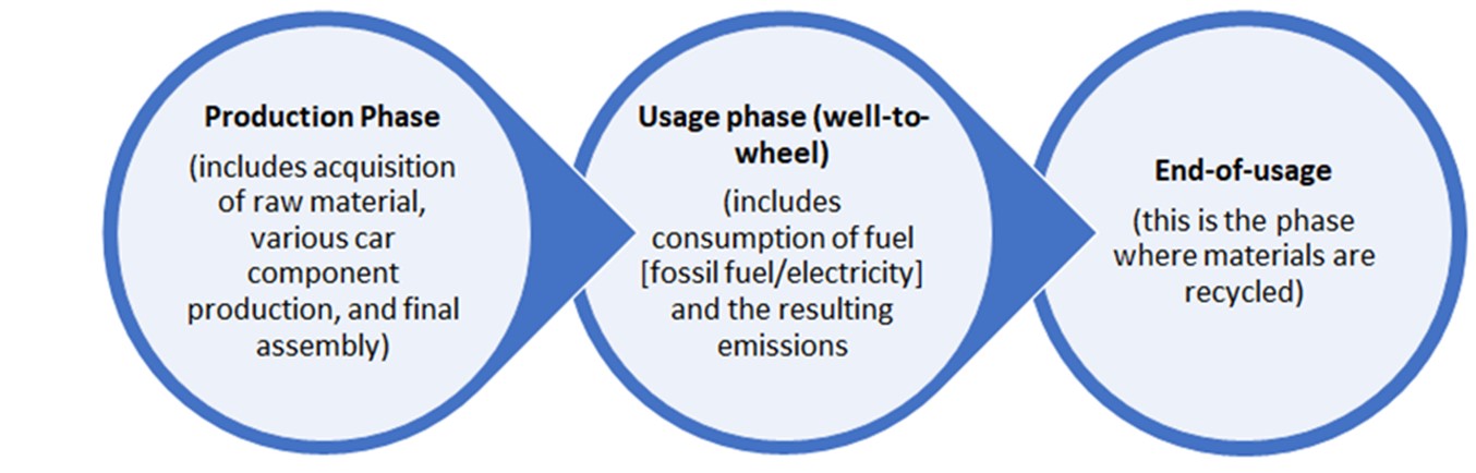
Below is a schematic showing the life-cycle for a typical EV from production to termination of usage. An EV, by its nature of production type as well as type of usage, typically have less carbon footprint in each lifecycle phase compared to that of a fossil fuel burning vehicle.
It is important to note that while PHEVs offer the potential for significant reduction in the usage of fossil fuel and resulting emissions of greenhouse gases, the actual benefit calculations need to take into account the upstream energy and emissions penalties that are associated with the electricity generation needed to power the charging systems and the load on the grid. Few studies have indeed taken all of these factors into account for certain vehicles that offer a choice of electric or internal combustion engine options for the same model. A study on the well known Volkswagen Golf model showed that, using the latest EU electricity mix, the current Golf TDI (Diesel) emits 140g CO2/km on average over its entire life cycle, while the e-Golf1 reaches 119g CO2/km. Based on the report, most of the emissions occur during the use phase of the internal combustion engine vehicle. Here the diesel reaches 111g CO2/km while a corresponding vehicle with electric drive emits only 62g CO2/km during the same phase [2].
Key findings about EV and carbon emission
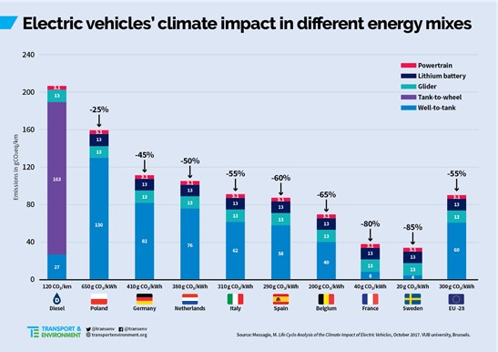
Several european countries where EVs are prevalent have significantly more carbon-intensive power generation – due to reliance on coal plants – EVs still perform better there on a lifecycle basis, which includes the emissions in manufacturing the battery and vehicle. Based on the Polish average, an EV emits 25% less CO2 over its lifetime. In Sweden, which has one of the cleanest energy mixes in the EU, an EV emits 85% less than a diesel car [3]. The figure below shows a summary of the study [3,4].
EV Climate impact for different Energy Mixes (reproduced from Transport and Environment)
Replacing a traditional ride-hailing car with an electric vehicle would deliver three times the environmental benefits and emission reductions, according to a new study. The finding comes as a new cost analysis shows that e-vehicles are cheaper to run for Uber drivers in many European cities, and Uber in Portugal says it will only take on new drivers if they have an EV.
Both Uber and Lyft have made recent statements expressing their intention to move towards a totally electric fleet. But now, for the first time, a study has looked at what the environmental impact might be. The study by University of California’s transportation institute, looked at 400,000 journeys made in a battery EV by 1,000 ride-hailing drivers, and compared the impact with 118,668 journeys made in a petrol or diesel car, as well as over 15,000 in a plug-in hybrid EV [5].
The biggest finding is that the potential environmental and emission reduction benefits of replacing a ride-hailing traditional car with an EV are ‘approximately three times higher compared with those of regular vehicle usage in California’, and on emissions alone this was ‘the most pessimistic scenario’. This is because vehicles owned by Uber, Lyft and other ride-hailing drivers are driven more than if they were only used for private use (about 305km on average per day compared to 48km) [5].
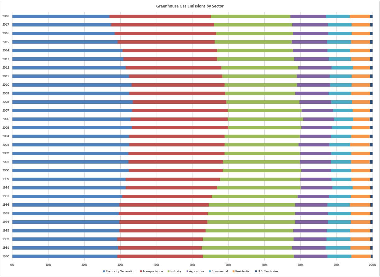
Below is a chart based on data from EPA in the US for greenhouse gas emissions by different sectors [9] . Based on the data, it can be seen that transportation sector contributes to a large amount of green house emission. It will be interesting to see the insights about how EVs and PHEVs come into play.
Share of Greenhouse Gas Emission by Sector
How to calculate carbon footprint:
Carbon offsetting funds solutions to reducing carbon emissions now. Frequently carbon offsetting reduces emissions much faster than you can as an individual/single company. Carbon offsetting projects help to combat global climate change as well as caring for local communities. In many instances providing much needed employment, health improvement, biodiversity, reforestation and broad social benefits to impoverished communities.
Calculator:
This free to use online carbon calculator tool is independently audited on an annual basis as part of the Quality Assurance Standard (QAS) for Carbon Offsetting.
Elgowainy, A., Burnham, A., Wang, M., Molburg, J., & Rousseau, A. (2009). Well-to-wheels energy use and greenhouse gas emissions of plug-in hybrid electric vehicles. SAE International Journal of Fuels and Lubricants, 2(1), 627-644.
Messagie, M. (2014). Life cycle analysis of the climate impact of electric vehicles. Journal of Life Cycle Assessment, 2014, 14.
Jenn, A. (2020). Emissions benefits of electric vehicles in Uber and Lyft ride-hailing services. Nature Energy, 5(7), 520-525.
Noori, M., Gardner, S., & Tatari, O. (2015). Electric vehicle cost, emissions, and water footprint in the United States: development of a regional optimization model. Energy, 89, 610-625.
When scientists or politicians begin to talk about climate change, most people become scared by the severity of the issue at hand, thinking there’s not a lot left for us to do. This fear-mongering tactic typically discourages individual actions like recycling or moving away from meat-focused diets. Scientists surely don’t want to scare the public with the truth, but the fact of the matter is that if we don’t do something now, our generation and all generations to follow will not have a safe or even comfortable planet to live on. This leads us to the question: what exactly can we do to prepare for and mitigate the coming decades of destruction and chaos?
The first step to approaching the threat of climate change is to understand the impact we’re facing. To do so, we consider contributing factors in their current capacity that are predicted to change; by observing these patterns early on, it will be easier to assess the risk to infrastructure and communities. Variables that have the capability to become dangerous in the future include global sea level, atmospheric temperatures, ocean acidification, and glacial stability [4, 6]. The severity of predicted impact depends on the response of all of these variables to atmospheric carbon dioxide and other pollutant levels that have already increased global temperature. Scientists anticipate a 68% likelihood of 1-4 feet of sea level rise as a result, with 10 feet being the worst case scenario [1, 4]. With these predictions come the growing probability of worse hurricane seasons due to increased storm surge and extreme precipitation [4]. Even now we see worsening severity of weather events compared to 20 years prior and flooding during high tides in areas below sea level [1].
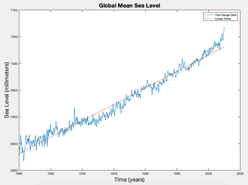
Global mean sea level since 1880 using tide gauge data from global PSMSL data base.
Conveniently, scientists have been monitoring sea level globally for nearly 200 years. However, gauging sea level is a bit more difficult than sticking a ruler somewhere on the coast and guessing the relative position over time. In 1807, Thomas Jefferson ordered a systematic survey utilizing “tide staffs”, or long poles that researchers used to compare sea level with a fixed point on nearby land [2]. It wasn’t until 1851 that the US coast guard implemented self recording tide gauges, but the device was still difficult to maintain and expensive to install [2]. Today’s advanced technology records the sea surface height via radar, or microwaves, with respect to the position of the gauge above the water. These gauges are a step up from acoustic gauges that must be protected from inclement weather, and cost upwards of $1300 [1, 2]. Although we have about 200 years of global sea level data, moving onto more reliable and cost efficient methods of measuring current and future sea level change is necessary for any chance of adaptation.
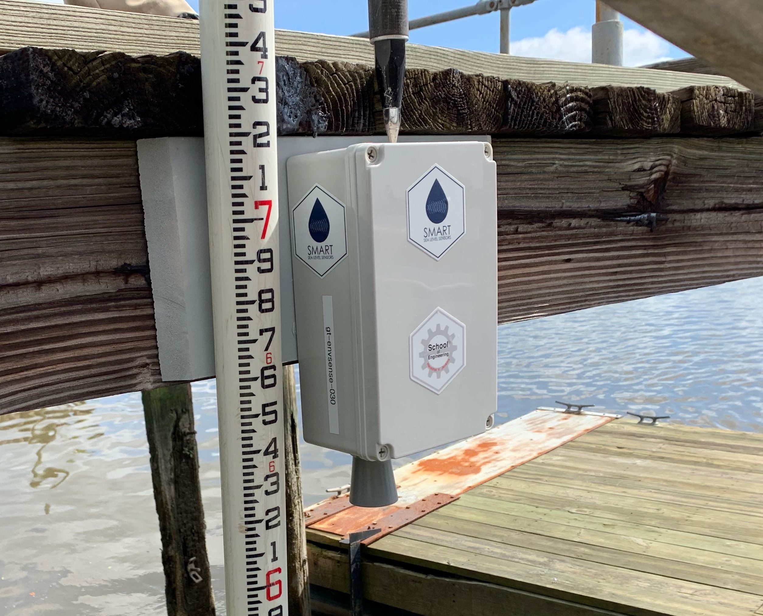
Dr. Kim Cobb and Dr. Russ Clark of Georgia Tech have spearheaded a project as a key initiative of the Global Change Program to provide low-cost tide gauges for Georgia coastlines. The Smart Sea Level venture is focused on particularly high risk regions, such as Chatham county. These $300 devices currently measure the relative sea level, air temperature, and barometric pressure, with planned capabilities to observe ocean properties, air quality, and inland flooding [5]. The smart sea level sensors use the roundtrip travel time of ultrasonic waves to measure the distance from the sensor to the water level. They log measurements every ten minutes, enabling their batteries to last one year or longer [5]. Already Georgia Tech scientists and collaborators can simulate tides, hurricanes, and extreme weather events via 43 strategically placed sensors [1, 5]. With this data, we’re moving towards predicting the flood patterns linked to severe weather events as atmospheric temperatures and sea levels continue to rise.
Smart Sea Level tide gauge adapted from Russ Clark of Georgia Tech.
As storm surge severity increases, so does the compounded risk of damaging communities beyond repair, which is the true threat of forthcoming extreme weather events. Many low income areas don’t have the resources to assist with evacuation or the infrastructure resilient enough to survive mass flooding. The smart sea level sensor project has led to close collaboration with these communities to provide information on the regions they’re most concerned with: air quality, temperature changes, and the future safety of family neighborhoods and K-12 school grounds [1]. Already the team has joined up with H. V. Jenkins School and Oglethorpe Charter Middle School [7] to recruit volunteers for engineering and installation, and test a climate literacy curriculum, respectively.
Now the question is to ask, what’s left to do? My personal answer would be to riot and do all we can to support this initiative, but that seems a little drastic. Increasing educational partnerships with high schools and elementary programs would improve awareness amongst the younger generations who are bound to be affected more by climate related concerns. Furthermore, getting into contact with legislators, particularly within the Georgia General Assembly would provide useful in terms of allocating funds towards this cause. With legislators on board, it’s possible legal action could be taken to prevent further damage towards vulnerable communities in areas like Chatham County. Programs such as incentivizing corporate relocation or the mitigation of current industrial hazards, could go a long way in establishing baselines for future climate change strategy. While most legislation to be passed will need to be from within the county, or even at the state level , it wouldn’t hurt to reach national recognition. By promoting climate literacy across the United States, we can increase the number of volunteers assisting with future adaptation, and motivate Congress to aid in the process of protecting these at risk communities [8].
If you’re interested in supporting this cause, check out the following volunteer and educational opportunities:
Cobb, K. (2019, January 24). Smart Sea Level Sensors – Chatham County. Retrieved from http://smartcities.gatech.edu/sites/default/files/GA-Smart-Webinar_Smart-Sea-Level-Sensors_1-24-2019.pdf
Dusto, A. (2014, August 4). Reading between the tides: 200 years of measuring global sea level: NOAA Climate.gov. Retrieved from https://www.climate.gov/news-features/climate-tech/reading-between-tides-200-years-measuring-global-sea-level
Georgia, S. (n.d.). Office of Sustainability. Retrieved from https://www.savannahga.gov/507/Office-of-Sustainability
Lindsey, R. (2019, November 19). Climate Change: Global Sea Level: NOAA Climate.gov. Retrieved from https://www.climate.gov/news-features/understanding-climate/climate-change-global-sea-level
Matthews, R., Cobb, K., & Clark, R. (2019). FAQ. Retrieved from https://www.sealevelsensors.org/faq/
Ocean Acidification. (n.d.). Retrieved from https://www.noaa.gov/education/resource-collections/ocean-coasts-education-resources/ocean-acidification
Jarvis, K. (2019, May 16). Smart Sea Sensors Expo Highlights Accomplishments and Shares Future Plans. Retrieved from https://www.news.gatech.edu/2019/05/16/smart-sea-sensors-expo-highlights-accomplishments-and-shares-future-plans
US Department of Commerce, & National Oceanic and Atmospheric Administration. (2005, December 19). NOS Education Offering. Retrieved from https://oceanservice.noaa.gov/education/literacy.html
Ever walk by an organic chemistry teaching lab and wonder why people were standing behind blowtorches looking frustrated?
First week of my senior year, I actually walked into that classroom.
In this class we learned a lot about organic and inorganic synthesis, lab techniques, and how to really think like chemists. It was much less structured than previous classes so a lot of times things wouldn’t go as expected and we had to troubleshoot the problems. These are all skills I expected to learn sometime in my Georgia Tech chemistry education, but there was one skill I never anticipated needing to master before graduation: glassblowing.
I don’t know why it never occurred to me that scientific glassblowing was a profession or even a position that universities frequently kept on staff but it didn’t. And that first day of class they announced a semester-long project where we would have to create 3 glass pieces for a grade.
At first we all shrugged, watched the demonstration, decided it didn’t look too difficult and gave it our first try. I’ve always considered myself a fairly artistic person so I figured it would be an easy grade buffer for what was shaping up to be a very difficult class. Boy was I wrong. The glass melted and curled in ways we didn’t expect, getting the right gas/oxygen ratio to have the right flame shape and heat was impossible, people burned themselves left and right and nothing we made came out to look anything like the simple demonstration she gave us. Frustrated and burned, the 10 of us muddled through the 4 hour demonstration and practice session with the professional glassblower and when she finally left we looked at our TAs in horror and asked, “will we need to be able to do this well if we ever want to be chemists?”.
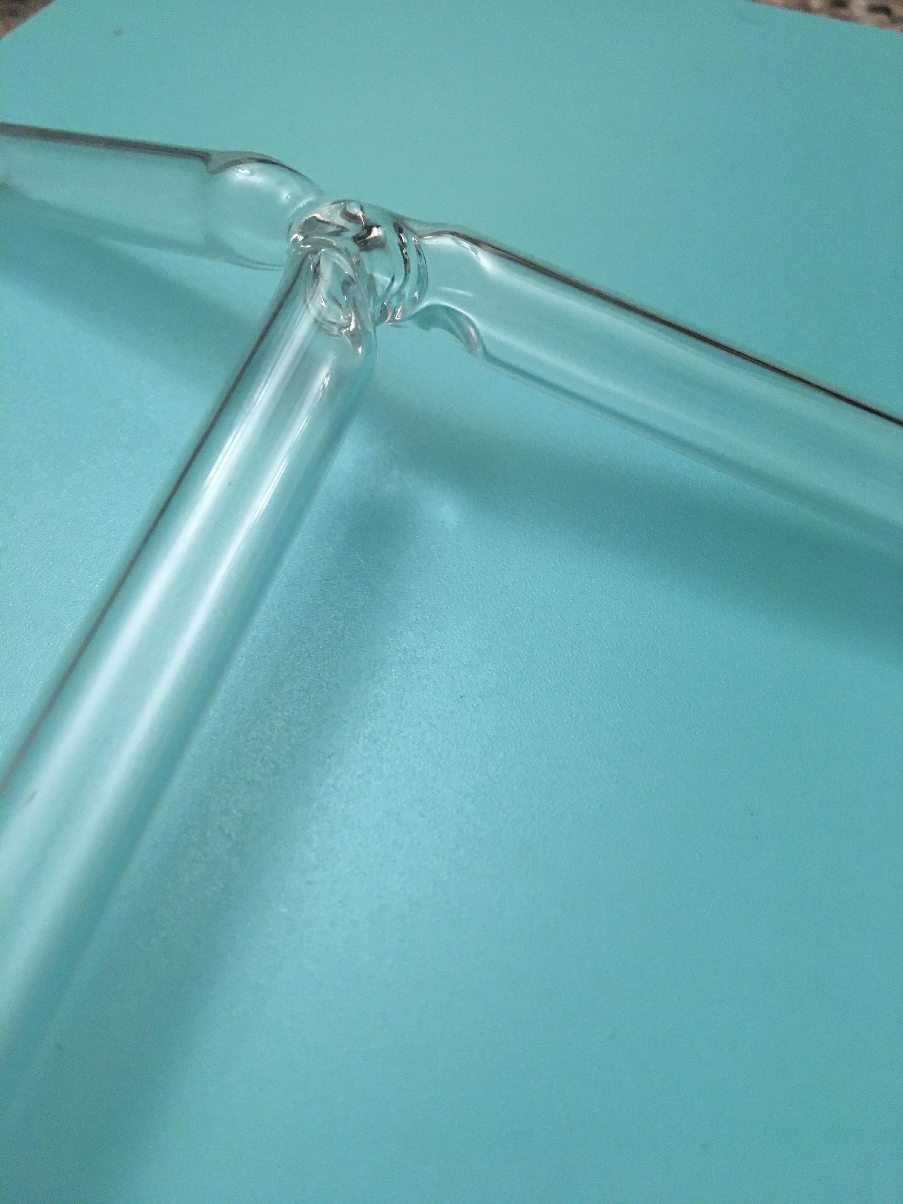
(10th attempt at a T-joint)
Their response? Laughter. What did we expect. They probably go through this every year with the new crop of students.
They told us that we wouldn’t need to be able to do this perfectly or really make custom glassware on a regular basis in order to be chemists. However, custom glassware was occasionally needed for experiments and one big point of the assignment was that we would then have an appreciation for what is and is not possible in glassblowing and just how difficult whatever we design would be to make. They also told us that even though as chemists we probably would never have to blow something as complicated as a Shlenck line ourselves, there is a very good chance we may need to have two pieces of glassware fused or a crack repaired and being able to quickly repair it yourself instead of waiting for a glassblower to get to your piece in a long line of work can be important to the success of a project up against a deadline.
So we worked on creating our three pieces: an ampule, a T-joint, and a straight seal. They didn’t have to be pretty but the ampule needed to be air-tight and all of the pieces had to be worked out to the point where you couldn’t tell they were once separate pieces of glass.
At the end of the semester, they loaded our ampules with [Co(NH3)5(ONO)]Cl2, a compound that changes color with prolonged air exposure, and had us seal them. Then we turned in our straight seals and T-joints.
Long story short? Glassblowing is much harder than I ever thought it would be. I will probably never have to do it on a regular basis, but this was an incredibly fun, if somewhat stressful, skill to have the opportunity to develop. And if I ever need to seal something airtight I’ll know how!